Mastering DNS Performance: Tools and Techniques for Optimizing Network Latency

In the previous section, we explored how to analyze and optimize DNS performance issues. To summarize, DNS acts as a mapping system between domain names and IP addresses, making it a widely used method for implementing Global Server Load Balancing (GSLB).

Typically, services exposed to the public internet are bound to a domain name. This not only makes it easier for people to remember but also prevents backend service IP changes from affecting users.

However, keep in mind that DNS resolution is subject to various network conditions and its performance may be unstable. For instance, increased public network latency, expired cache requiring upstream server requests, or inadequate DNS server performance during high traffic periods can all cause delays in DNS responses.

During such instances, you can use debugging tools like nslookup or dig to analyze the DNS resolution process and pair them with tools like ping to debug latency issues to the DNS server, thereby pinpointing performance bottlenecks. Methods like caching, prefetching, or using HTTPDNS can often be employed to optimize DNS performance.

In the last section, we used ping, which is one of the most common tools for testing service latency. In many cases, ping can help identify latency issues. However, there are instances where ping itself might exhibit unexpected behavior, necessitating the need to capture the sent and received packets of the ping command and analyze these packets to identify the root cause of the issue.

Tools like tcpdump and Wireshark are indispensable for packet capture and network performance analysis.

• 
  

  tcpdump is a command-line-based tool used primarily on servers for capturing and analyzing network packets.

  
  
• 
  

  Wireshark, aside from packet capturing, provides a powerful graphical interface and summary analysis features, making it especially convenient for analyzing complex network scenarios.

  
  

Therefore, in practical network performance analyses, it is a common practice to first use tcpdump for packet capture and then analyze the data with Wireshark.

Today, I’ll walk you through how to use tcpdump and Wireshark to analyze network performance issues.

Case Preparation

This tutorial is based on Ubuntu 18.04, but the same steps apply to other Linux systems. I’m using the following setup for this demonstration:

• 
  

  Machine configuration: 2 CPUs, 8GB of memory.

  
  
• 
  

  Preinstalled tools: tcpdump, Wireshark, etc., as shown:

  
  

# For Ubuntu
apt-get install tcpdump wireshark

# For CentOS
yum install -y tcpdump wireshark

Since Wireshark is a graphical tool, you can’t use it over SSH. It’s recommended to install it on your local machine (e.g., Windows). You can download and install Wireshark from https://www.wireshark.org/.

As before, all commands used in the case are run as the root user (except in Windows when running Wireshark). If you are logged in as a regular user, switch to the root user by running sudo su root.

Re-exploring ping

As introduced earlier, ping is one of the most commonly used network tools for testing connectivity and latency between network hosts. The concepts and usage of ping were briefly covered in the Linux Networking Basics. Additionally, in cases of slow DNS responses, ping was used multiple times to measure DNS server latency (RTT).

However, although ping is quite simple, sometimes you may notice anomalies in its behavior. For instance, it could appear slow even though the actual network latency is low.

Let’s begin by opening a terminal, SSH into the example machine, and run the following command to test connectivity and latency with Geekbang Tech’s official website. If everything is normal, you’ll see an output like the one below:

# Ping 3 times (default sending interval is 1 second)
# Assume the DNS server is still configured as 114.114.114.114
$ ping -c3 geektime.org
PING geektime.org (35.190.27.188) 56(84) bytes of data.
64 bytes from 35.190.27.188 (35.190.27.188): icmp_seq=1 ttl=43 time=36.8 ms
64 bytes from 35.190.27.188 (35.190.27.188): icmp_seq=2 ttl=43 time=31.1 ms
64 bytes from 35.190.27.188 (35.190.27.188): icmp_seq=3 ttl=43 time=31.2 ms

--- geektime.org ping statistics ---
3 packets transmitted, 3 received, 0% packet loss, time 11049ms
rtt min/avg/max/mdev = 31.146/33.074/36.809/2.649 ms

The interpretation of ping output was discussed in the Linux Networking Basics, which you can revisit to analyze this output yourself.

Note, if your ping completes unusually quickly, try executing the following command and then retry. We’ll explain the meaning of this command later.

# Drop packets from the DNS server containing "googleusercontent"
$ iptables -I INPUT -p udp --sport 53 -m string --string googleusercontent --algo bm -j DROP

From the ping output, you can observe that after resolving geektime.org, its IP address is 35.190.27.188. All three ping requests received responses with an RTT of around 30ms.

However, look at the summary section—it gets interesting. There were 3 transmissions and 3 responses with no packet loss, yet the total time for sending and receiving these packets exceeded 11 seconds (11049ms), which seems puzzling.

Thinking back to the previous DNS resolution issue, you’d suspect this might be a slow DNS resolution. But is it?

Looking closer at the ping output, we see that all three ping requests used an IP address directly, meaning DNS resolution only occurred when the command initially executed.

Let’s confirm this with nslookup. Execute the following command in the terminal and include the time command to measure the execution time of nslookup:

$ time nslookup geektime.org
Server: 114.114.114.114
Address: 114.114.114.114#53

Non-authoritative answer:
Name: geektime.org
Address: 35.190.27.188


real    0m0.044s
user    0m0.006s
sys     0m0.003s

The DNS resolution is indeed very fast—only 44ms, which is significantly shorter than 11 seconds.

At this point, how do we proceed with further analysis? This is where tcpdump becomes useful to capture packets and verify what ping is actually transmitting and receiving.

Open another terminal (Terminal 2), SSH into the example machine, and execute the following command:

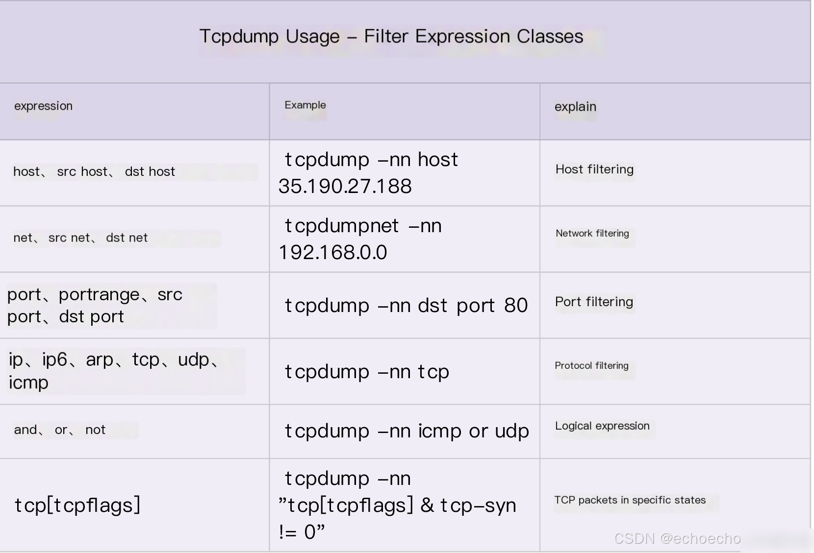
$ tcpdump -nn udp port 53 or host 35.190.27.188

While you could run tcpdump without any parameters, it would capture many irrelevant packets. Since we already ran the ping command earlier and know that geektime.org resolves to 35.190.27.188 and involves DNS queries, we add specific filters to refine the capture output with the above command.

Here’s a breakdown of this command:

• 
  

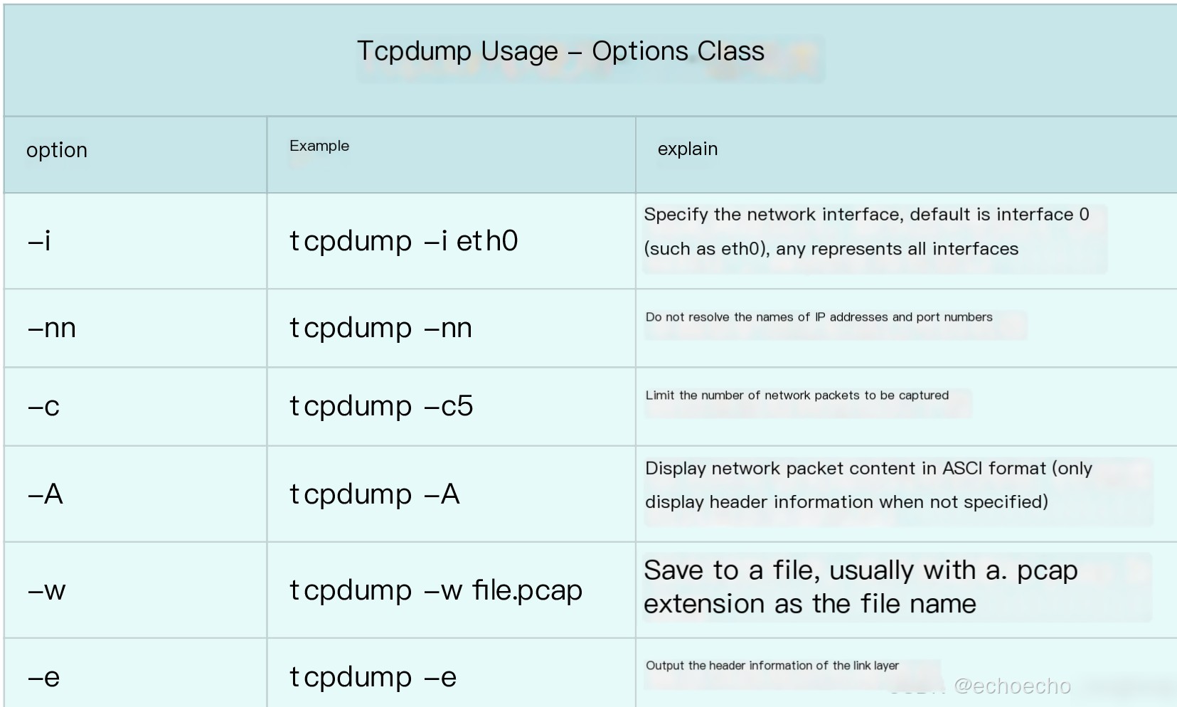
  -nn: Disables resolution of domain names, protocols, and port numbers in the captured packets.

  
  
• 
  

  udp port 53: Captures only packets using the UDP protocol with source or destination port 53 (commonly used for DNS).

  
  
• 
  

  host 35.190.27.188: Filters packets with source or destination IP address 35.190.27.188.

  
  
• 
  

  The or operator combines the above filters, so matching either condition will display relevant packets.

  
  

Next, return to Terminal 1 and rerun the same ping command:

$ ping -c3 geektime.org
...
--- geektime.org ping statistics ---
3 packets transmitted, 3 received, 0% packet loss, time 11095ms
rtt min/avg/max/mdev = 81.473/81.572/81.757/0.130 ms

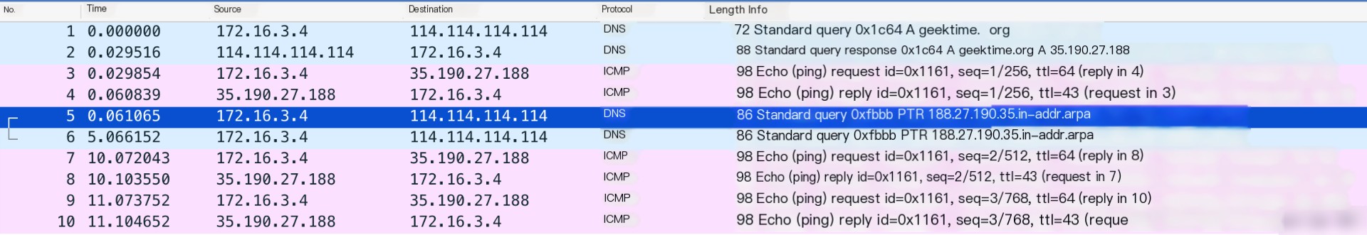
After completing the command, review the tcpdump output in Terminal 2:

tcpdump: verbose output suppressed, use -v or -vv for full protocol decode
listening on eth0, link-type EN10MB (Ethernet), capture size 262144 bytes
14:02:31.100564 IP 172.16.3.4.56669 >  114.114.114.114.53: 36909+ A? geektime.org. (30)
14:02:31.507699 IP 114.114.114.114.53 >  172.16.3.4.56669: 36909 1/0/0 A 35.190.27.188 (46)
14:02:31.508164 IP 172.16.3.4 >  35.190.27.188: ICMP echo request, id 4356, seq 1, length 64
14:02:31.539667 IP 35.190.27.188 >  172.16.3.4: ICMP echo reply, id 4356, seq 1, length 64
14:02:31.539995 IP 172.16.3.4.60254 >  114.114.114.114.53: 49932+ PTR? 188.27.190.35.in-addr.arpa. (44)
14:02:36.545104 IP 172.16.3.4.60254 >  114.114.114.114.53: 49932+ PTR? 188.27.190.35.in-addr.arpa. (44)
14:02:41.551284 IP 172.16.3.4 >  35.190.27.188: ICMP echo request, id 4356, seq 2, length 64
14:02:41.582363 IP 35.190.27.188 >  172.16.3.4: ICMP echo reply, id 4356, seq 2, length 64
14:02:42.552506 IP 172.16.3.4 >  35.190.27.188: ICMP echo request, id 4356, seq 3, length 64
14:02:42.583646 IP 35.190.27.188 >
``````html

In this output, the first two lines indicate the options and basic interface information for tcpdump. Starting from the third line, the captured network packet output is displayed. The format of these outputs generally follows this structure: timestamp protocol source_address.source_port > destination_address.destination_port packet_details. This is the most basic format, though additional fields can be included via options.

 

The initial fields are relatively straightforward to understand. However, the packet details depend on the specific protocol in question. Therefore, fully understanding the meaning of captured network packets requires a foundational knowledge of common network protocol formats and their interaction principles.

 

Of course, much of this information is documented in the RFCs (Request for Comments) published by the Internet Engineering Task Force (IETF). You can view the RFC index here.

 

For example, the first line indicates an A record query request sent from the local IP to 114.114.114.114. This message format is documented in RFC1035. In this specific tcpdump output:

• 
  

  36909+ represents the query ID. It will also appear in the response, and the plus sign indicates recursion is enabled.

  
  
• 
  

  A? represents an A record query.

  
  
• 
  

  geektime.org. is the queried domain name.

  
  
• 
  

  30 indicates the message’s length.

  
  

The subsequent line is the DNS response from 114.114.114.114, stating that the A record of geektime.org. resolves to 35.190.27.188.

 

The third and fourth lines represent an ICMP echo request and its corresponding echo reply. By subtracting the request timestamp (14:02:31.508164) from the response timestamp (14:02:31.539667), the ICMP round-trip time is calculated to be 30 ms, which appears normal.

 

However, the following two lines regarding PTR (reverse address lookup) requests are more suspicious. These requests only display outgoing packets but no responses. Closer inspection of their timestamps reveals that each request results in a 5-second delay before the next network packet, with the two PTR requests cumulatively consuming 10 seconds.

 

Further down, there are four additional packets that represent two normal ICMP requests and their corresponding replies. The calculated delay for these exchanges is also 30 ms.

 

At this point, the root cause of the sluggish ping performance is identified: the two unacknowledged PTR requests result in timeouts. PTR reverse lookup queries are designed to map an IP address to a hostname, but not all IP addresses have a defined PTR record, meaning the query might fail.

 

As a result, if you experience slow ping command execution despite low latency, it is likely the PTR lookups causing the delay.

 

Resolving the issue is straightforward—disable PTR queries. As usual, consult the ping manual by running man ping to find the appropriate option. Adding the -n flag disables name resolution. For example, you can execute the following command in your terminal:

$ ping -n -c3 geektime.org
PING geektime.org (35.190.27.188) 56(84) bytes of data.
64 bytes from 35.190.27.188: icmp_seq=1 ttl=43 time=33.5 ms
64 bytes from 35.190.27.188: icmp_seq=2 ttl=43 time=39.0 ms
64 bytes from 35.190.27.188: icmp_seq=3 ttl=43 time=32.8 ms

--- geektime.org ping statistics ---
3 packets transmitted, 3 received, 0% packet loss, time 2002ms
rtt min/avg/max/mdev = 32.879/35.160/39.030/2.755 ms

Notice how the execution time has dropped dramatically to 2 seconds from the previous 11 seconds.

Using tcpdump, we successfully diagnosed and resolved a common ping performance issue.

At the end of the case, if you executed an iptables command earlier, remember to delete the rule:

$ iptables -D INPUT -p udp --sport 53 -m string --string googleusercontent --algo bm -j DROP

Nonetheless, you might still wonder why the filter included the unrelated string googleusercontent, given our case involves no Google-related issues.

In reality, switching to a different DNS server can provide a PTR result for 35.190.27.188, as shown below:

$ nslookup -type=PTR 35.190.27.188 8.8.8.8
Server:	8.8.8.8
Address:	8.8.8.8#53
Non-authoritative answer:
188.27.190.35.in-addr.arpa	name = 188.27.190.35.bc.googleusercontent.com.
Authoritative answers can be found from:

As you see, the PTR record maps to 188.27.190.35.bc.googleusercontent.com rather than geektime.org. This explains why the initial iptables rule targeting googleusercontent dropped the PTR responses, resulting in timeouts.

tcpdump is undoubtedly a powerful tool for network performance analysis. Next, I’ll walk you through more advanced tcpdump usage techniques.

tcpdump

As you know, tcpdump is one of the most commonly used network analysis tools. It leverages the libpcap library and Linux’s AF_PACKET socket to capture packets traveling through a network interface. Combined with its robust filtering options, it allows you to extract precisely the information you’re interested in from a torrent of packet data.

While tcpdump provides meticulous details for each packet, this means a prerequisite understanding of network protocols is required. To bridge this gap, the most authoritative resources for protocol specifics are the RFCs available here.

However, RFCs can be intimidating for beginners. If you’re relatively new to network protocols, I recommend starting with “TCP/IP Illustrated, Volume 1: The Protocols.” This is an essential foundation for every programmer.

Back to tcpdump, its basic usage follows this syntax:

tcpdump [options] [filter_expression]

The square brackets denote that both options and filter expressions are optional.

Tip: In Linux tools, when you see options enclosed in square brackets in a document, it signifies that those options are optional. Be mindful of whether default values exist in these cases.

Referencing the tcpdump manual and the pcap-filter manual, you’ll find a plethora of options and filter expressions available. Don’t be overwhelmed—mastering a subset of commonly used options and filters is sufficient for most scenarios.

To help you get started quickly, I’ve compiled some of the most common usage patterns into tables. First, let’s review frequently used options. In the earlier ping case, we used the -nn option to disable IP and port name resolution. Additional commonly used options are explained in the following table:

Next, let’s discuss frequently used filter expressions. In the previous example, we used udp port 53 or host 35.190.27.188 to capture DNS protocol packets and packets with a source or destination address of 35.190.27.188. Additional examples are summarized below:

Finally, a quick recap of the tcpdump output format:

timestamp protocol source_address.source_port > destination_address.destination_port packet_details

The packet details are protocol-specific, meaning their format varies depending on the protocol in question. For more detailed usage styles, consult the tcpdump manual (run man tcpdump on the command line).

That said, while tcpdump is incredibly powerful, its output isn’t particularly user-friendly. Specifically, when dealing with a high volume of packets (e.g., tens of thousands per second), analyzing problems becomes cumbersome.

In contrast, Wireshark offers a graphical user interface (GUI) coupled with a suite of summary and analysis tools, enabling you to address network performance issues more efficiently. Let’s delve into it next.

Wireshark

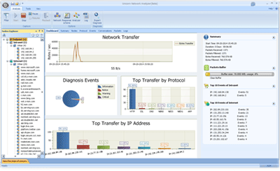
Wireshark is one of the most popular network analysis tools, and its primary advantage lies in its cross-platform graphical interface. Like tcpdump, Wireshark provides powerful filter rules but also incorporates a variety of summary and analysis tools.

As an example, consider the earlier ping case. Save the captured packets into a ping.pcap file using:

$ tcpdump -nn udp port 53 or host 35.190.27.188 -w ping.pcap

Then, transfer the file to a machine running Wireshark. For instance, you can use scp to move it locally:

$ scp host-ip/path/ping.pcap .

Once transferred, open the file in Wireshark. The graphical interface will resemble the following:

“`Here’s the translated content of your WordPress post while preserving the original structure, HTML tags, and formatting intact:

—

From Wireshark’s interface, you can observe that it not only displays the headers of network packets in a more organized format but also uses different colors to distinguish between DNS and ICMP protocols. You can easily spot that the two PTR queries in the middle did not receive response packets.

Next, after selecting a specific packet from the network packet list, you’ll notice that the packet details section beneath it shows detailed information about the layers within the protocol stack. For example, let’s take a look at PTR packet number 5:

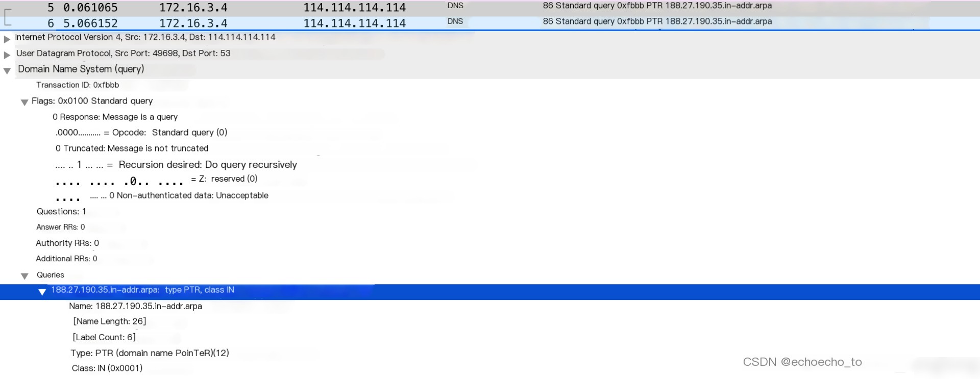
You’ll find the source and destination addresses in the Internet Protocol (IP) layer, details of the User Datagram Protocol (UDP) in the transport layer, and summary information of the Domain Name System (DNS) protocol in the application layer.

By clicking the arrow on the left side of each layer, you can view all the fields in that protocol’s header. For instance, clicking DNS will reveal specific fields such as Transaction ID, Flags, Queries, and their respective values and meanings.

Of course, Wireshark’s capabilities go far beyond this. Next, let’s explore an example using HTTP and understand the concepts of TCP’s three-way handshake and four-way termination.

In this example, we’ll access the Example Domain. First, in terminal one, execute the following command to retrieve the IP address of example.com. Then use the tcpdump command to filter traffic for the obtained IP address and save the results in a file named web.pcap:

 $ dig +short example.com
93.184.216.34
$ tcpdump -nn host 93.184.216.34 -w web.pcap

In fact, you can use the domain name directly in the host expression, as in `tcpdump -nn host example.com -w web.pcap`.

Next, switch to terminal two and execute the curl command below to visit Example Domain:

 $ curl http://example.com

Finally, switch back to terminal one, hit Ctrl+C to stop tcpdump, and extract the web.pcap file that’s been generated.

Open the web.pcap file with Wireshark, and you’ll see an interface like this:

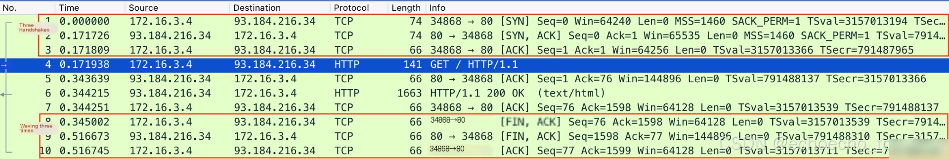
Since HTTP runs over TCP, the first three packets in the capture represent the three-way handshake. The following packets in the middle are the HTTP request and response packets, while the last three packets represent the TCP connection closure using a “three-way termination.”

From the menu bar, go to Statistics -> Flow Graph. In the pop-up window, select `TCP Flows` under Flow type to visualize the TCP flow execution process clearly:

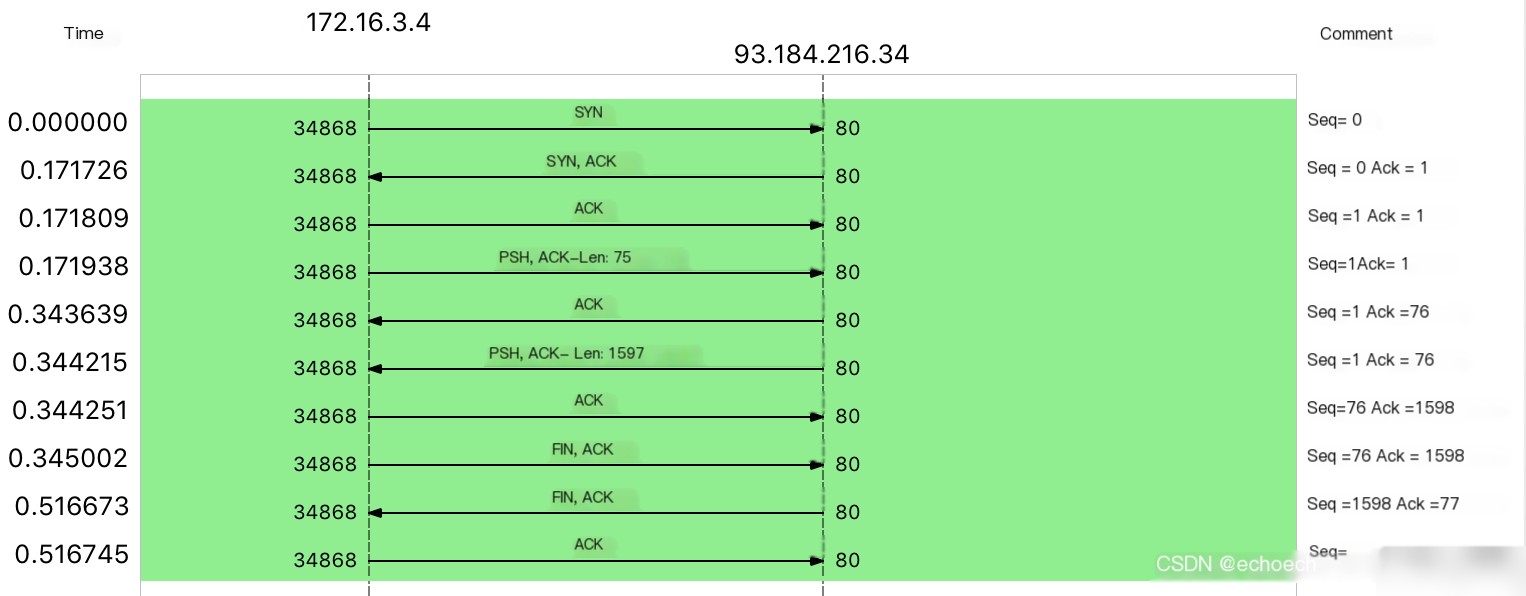
This is quite similar to the TCP three-way handshake and four-way termination diagrams you typically see in tutorials. For comparison, here’s a common illustration of these processes:

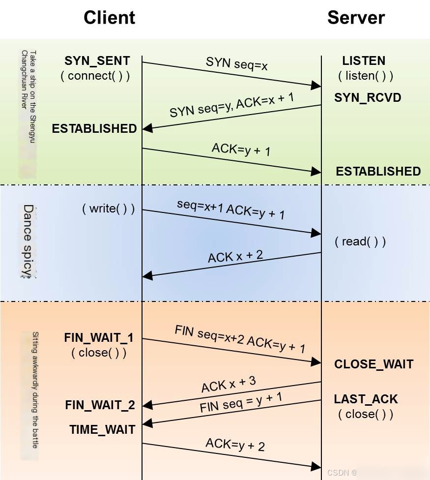
(Image source: CoolShell)

However, if you compare the two diagrams, you’ll notice that the packet capture here doesn’t completely align with the four-way termination description. Instead, the termination process involves only three packets rather than four.

The reason for having three packets is that after the server receives the FIN from the client, it simultaneously terminates the connection on its end. This allows it to combine the ACK and FIN into a single packet, saving one transmission and creating the “three-way termination.”

Typically, when the server receives the client’s FIN, it may not have finished sending all outgoing data. In such cases, it first replies with an ACK and waits until all data has been sent before sending the FIN, resulting in the conventional four-way termination.

After capturing packets, the interface in Wireshark, in the case of a four-way termination, looks like this (the raw network packet data is from the Wireshark TCP 4-times close example, and you can download it by clicking here):

Of course, the use of Wireshark doesn’t stop here. Explore more functionalities by visiting the official documentation and the Wireshark Wiki.

Summary

Today, we learned how to use tcpdump and Wireshark through several examples. These tools can help you analyze network communication processes and uncover potential performance issues.

If you realize that the same network service responds quickly using an IP address but is significantly slower when using a domain name, it could indicate DNS issues. DNS resolution doesn’t just include A-record requests to map domain names to IP addresses; in some cases, performance analysis tools make “smart” PTR requests to reverse-map IP addresses back to domain names.

Often, reverse-mapping an IP address to a domain name or resolving port numbers to protocol names is the default behavior of many network tools. However, this can slow down these performance tools. To mitigate this, most network performance tools offer options (e.g., `-n` or `-nn`) to disable name resolution.

In your work, when faced with network performance issues, don’t forget about the power of tcpdump and Wireshark. Use these tools to capture actual transmitted packets and diagnose performance problems efficiently.

Discussion

Finally, I’d like to hear your thoughts. How do you use tcpdump and Wireshark? Have you resolved specific network issues with these tools? How did you go about diagnosing, analyzing, and solving the problem? Feel free to incorporate what we’ve learned today and share your workflow.

I welcome your discussion in the comments section, and feel free to share this article with your colleagues and friends. Let’s learn through practice and grow through collaboration!

—

If you need additional adjustments or terminology details, let me know!